What’s new for SQL Server 2019 Analysis Services CTP 2.3
We find great pleasure in announcing the public CTP 2.3 of SQL Server 2019 Analysis Services. New features detailed here are planned to ship later in Power BI Premium and Azure Analysis Services.
Calculation groups
Here is a question for seasoned BI professionals: what is the most powerful feature of SSAS multidimensional? Many would say the ability to define calculated members, typically using scoped cell assignments. Calculated members in multidimensional enable complex calculations by reusing calculation logic. Unfortunately, Analysis Services tabular doesn’t have equivalent functionality. Correction: it does now!!!
Calculation groups address the issue of proliferation of measures in complex BI models often caused by common calculations like time-intelligence. Enterprise models are reused throughout large organizations, so they grow in scale and complexity. It is not uncommon for Analysis Services models to have hundreds of base measures. Each base measure often requires the same time-intelligence analysis. For example, Sales and Order Count may require:
- Sales MTD, Sales QTD, Sales YTD, Sales PY, Sales YOY%, …
- Orders MTD, Orders QTD, Orders YTD, Orders PY, Orders YOY%, …
As you can see, this can easily explode the number of measures. If a model has 100 base measures and each requires 10 time-intelligence representations, the model ends up with 1,000 measures in total (100*10). This creates the following problems.
- The user experience is overwhelming because must sift through so many measures
- DAX is difficult to maintain
- Model metadata is bloated
Calculation groups address these issues. They are presented to end-users as a table with a single column. Each value in the column represents a reusable calculation that can be applied to any of the measures where it makes sense. The reusable calculations are called calculation items.
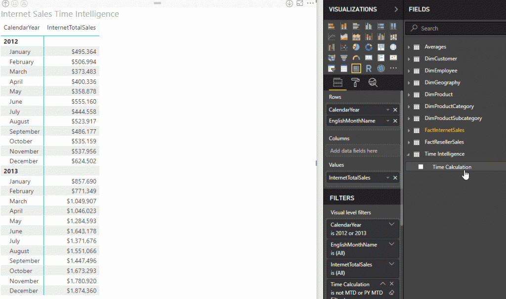
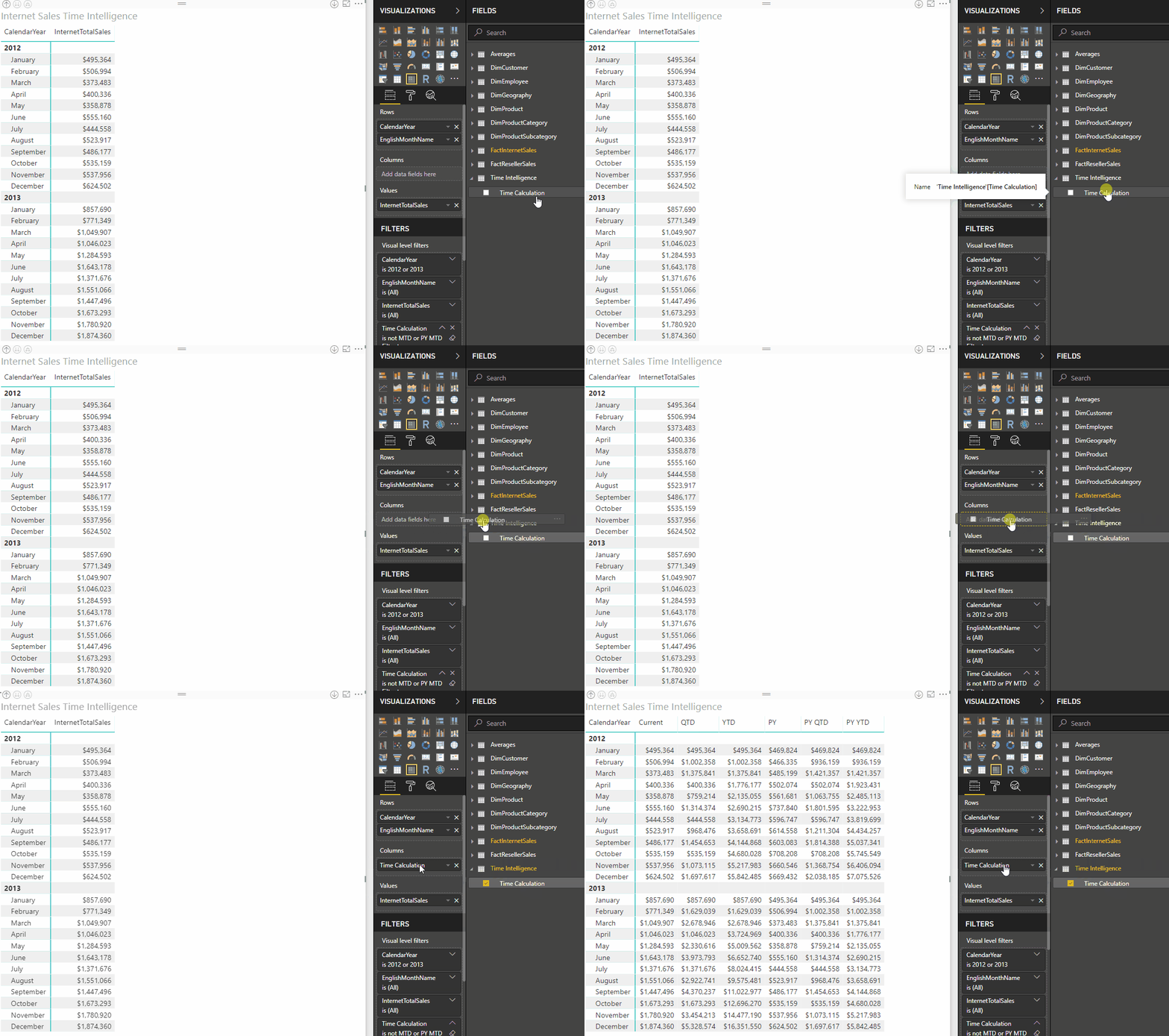
By reducing the number of measures, calculation groups present an uncluttered user interface to end users. They are an elegant way to manage DAX business logic. Users simply select calculation groups in the field list to view the calculations in Power BI visuals. There is no need for the end user or modeler to create separate measures.
Time-intelligence example
Consider the following calculation group example.
| Table | Time Intelligence |
| Column | Time Calculation |
| Precedence | 20 |
| Calculation Item | Expression |
"Current"
|
SELECTEDMEASURE()
|
"MTD"
|
CALCULATE(SELECTEDMEASURE(), DATESMTD(DimDate[Date])) |
"QTD"
|
CALCULATE(SELECTEDMEASURE(), DATESQTD(DimDate[Date])) |
"YTD"
|
CALCULATE(SELECTEDMEASURE(), DATESYTD(DimDate[Date])) |
"PY"
|
CALCULATE(SELECTEDMEASURE(), SAMEPERIODLASTYEAR(DimDate[Date])) |
"PY MTD"
|
CALCULATE( SELECTEDMEASURE(), SAMEPERIODLASTYEAR(DimDate[Date]), 'Time Intelligence'[Time Calculation] = "MTD" ) |
"PY QTD"
|
CALCULATE( SELECTEDMEASURE(), SAMEPERIODLASTYEAR(DimDate[Date]), 'Time Intelligence'[Time Calculation] = "QTD" ) |
"PY YTD"
|
CALCULATE( SELECTEDMEASURE(), SAMEPERIODLASTYEAR(DimDate[Date]), 'Time Intelligence'[Time Calculation] = "YTD" ) |
"YOY"
|
SELECTEDMEASURE() – CALCULATE( SELECTEDMEASURE(), 'Time Intelligence'[Time Calculation] = "PY" ) |
"YOY%"
|
DIVIDE( CALCULATE( SELECTEDMEASURE(), 'Time Intelligence'[Time Calculation]="YOY" ), CALCULATE( SELECTEDMEASURE(), 'Time Intelligence'[Time Calculation]="PY" ), ) |
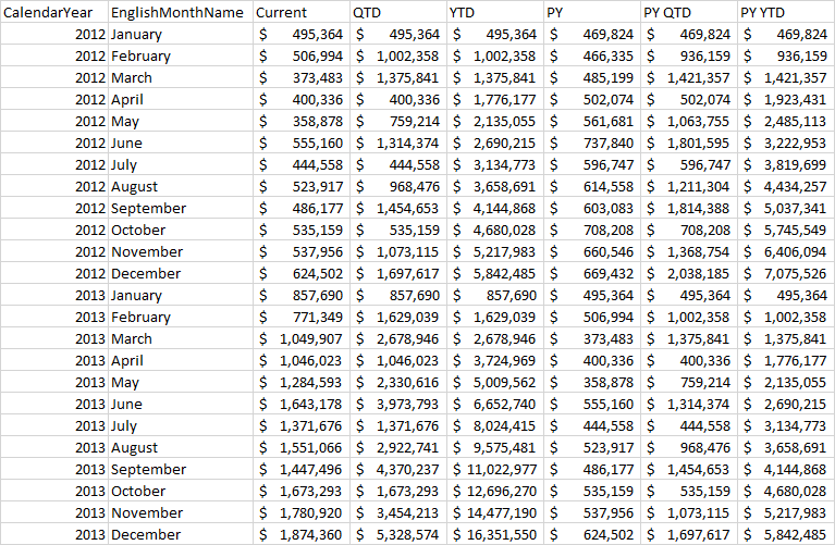
Here is a DAX query and output. The output shows the calculations applied. For example, QTD for March 2012 is the sum of January, February and March 2012.
EVALUATE
CALCULATETABLE (
    SUMMARIZECOLUMNS (
        DimDate[CalendarYear],
        DimDate[EnglishMonthName],
        "Current", CALCULATE ( [InternetTotalSales], 'Time Intelligence'[Time Calculation] = "Current" ),
        "QTD",     CALCULATE ( [InternetTotalSales], 'Time Intelligence'[Time Calculation] = "QTD" ),
        "YTD",     CALCULATE ( [InternetTotalSales], 'Time Intelligence'[Time Calculation] = "YTD" ),
        "PY",      CALCULATE ( [InternetTotalSales], 'Time Intelligence'[Time Calculation] = "PY" ),
        "PY QTD",  CALCULATE ( [InternetTotalSales], 'Time Intelligence'[Time Calculation] = "PY QTD" ),
        "PY YTD",  CALCULATE ( [InternetTotalSales], 'Time Intelligence'[Time Calculation] = "PY YTD" )
    ),
    DimDate[CalendarYear] IN { 2012, 2013 }
)
Sideways recursion
Some of the calculation items refer to other ones in the same calculation group. This is called “sideways recursion”. For example, YOY% (shown below for easy reference) refers to 2 other calculation items, but they are evaluated separately using different calculate statements. Other types of recursion are not supported (see below).
DIVIDE(
    CALCULATE(
        SELECTEDMEASURE(),
        'Time Intelligence'[Time Calculation]="YOY"
    ),
    CALCULATE(
        SELECTEDMEASURE(),
        'Time Intelligence'[Time Calculation]="PY"
    ),
)
Single calculation item in filter context
Here is the definition of PY YTD:
CALCULATE(
    SELECTEDMEASURE(),
    SAMEPERIODLASTYEAR(DimDate[Date]),
    'Time Intelligence'[Time Calculation] = "YTD"
)
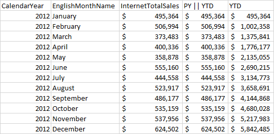
The YTD argument to the CALCULATE() function overrides the filter context to reuse the logic already defined in the YTD calculation item. It is not possible to apply both PY and YTD in a single evaluation. Calculation groups are only applied if a single calculation item from the calculation group is in filter context.
This is illustrated by the following query and output.
EVALUATE
CALCULATETABLE (
    SUMMARIZECOLUMNS (
        DimDate[CalendarYear],
        DimDate[EnglishMonthName],

        //No time intelligence applied: all calc items in filter context:
        "InternetTotalSales", [InternetTotalSales],

        //No time intelligence applied: 2 calc items in filter context:
        "PY || YTD", CALCULATE ( [InternetTotalSales],
            'Time Intelligence'[Time Calculation] = "PY" || 'Time Intelligence'[Time Calculation] = "YTD"
        ),

        //YTD applied: exactly 1 calc item in filter context:
        "YTD", CALCULATE ( [InternetTotalSales], 'Time Intelligence'[Time Calculation] = "YTD" )
    ),
    DimDate[CalendarYear] = 2012
)
A calculation group should be designed so that each calculation item within it presented to the end user only makes sense to be applied one at a time. If there is a business requirement to allow the end user to apply more than one calculation item at a time, multiple calculation groups should be used with different precedence.
Precedence
In the same model as the time-intelligence example above, the following calculation group also exists. It contains average calculations that are independent of traditional time intelligence in that they don’t change the date filter context; they just apply average calculations within it.
In this example, a daily average calculation is defined. It is common in oil-and-gas applications to use calculations such as “barrels of oil per day”. Other common business examples include “store sales average” in the retail industry.
Whilst such calculations are calculated independently of time-intelligence calculations, there may well be a requirement to combine them. For example, the end-user might want to see “YTD barrels of oil per day” to view the daily-oil rate from the beginning of the year to the current date. In this scenario, precedence should be set for calculation items.
| Table | Averages |
| Column | Average Calculation |
| Precedence | 10 |
| Calculation Item | Expression |
"No Average"
|
SELECTEDMEASURE()
|
"Daily Average"
|
DIVIDE(SELECTEDMEASURE(), COUNTROWS(DimDate)) |
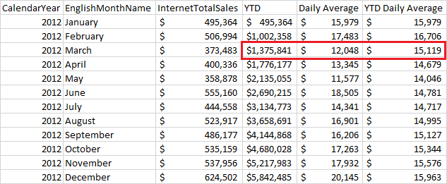
Here is a DAX query and output.
EVALUATE
    CALCULATETABLE (
        SUMMARIZECOLUMNS (
        DimDate[CalendarYear],
        DimDate[EnglishMonthName],
        "InternetTotalSales", CALCULATE (
            [InternetTotalSales],
            'Time Intelligence'[Time Calculation] = "Current",
            'Averages'[Average Calculation] = "No Average"
        ),
        "YTD", CALCULATE (
            [InternetTotalSales],
            'Time Intelligence'[Time Calculation] = "YTD",
            'Averages'[Average Calculation] = "No Average"
        ),
        "Daily Average", CALCULATE (
            [InternetTotalSales],
            'Time Intelligence'[Time Calculation] = "Current",
            'Averages'[Average Calculation] = "Daily Average"
        ),
        "YTD Daily Average", CALCULATE (
            [InternetTotalSales],
            'Time Intelligence'[Time Calculation] = "YTD",
            'Averages'[Average Calculation] = "Daily Average"
        )
    ),
    DimDate[CalendarYear] = 2012
)
The following table shows how the March 2012 values are calculated.
| Column name | Calculation |
| YTD | Sum of InternetTotalSales for Jan, Feb, Mar 2012
= 495,364 + 506,994 + 373,483 |
| Daily Average | InternetTotalSales for Mar 2012 divided by # of days in March
= 373,483 / 31 |
| YTD Daily Average | YTD for Mar 2012 divided by # of days in Jan, Feb and Mar
= 1,375,841 / (31 + 29 + 31) |
For easy reference, here is the definition of the YTD calculation item. It is applied with Precedence of 20.
CALCULATE(SELECTEDMEASURE(), DATESYTD(DimDate[Date]))
Here is Daily Average. It is applied with Precedence of 10.
DIVIDE(SELECTEDMEASURE(), COUNTROWS(DimDate))
Since the precedence of the Time Intelligence calculation group is higher than the Averages one, it is applied as broadly as possible. The YTD Daily Average calculation applies YTD to both the numerator and the denominator (count of days) of the daily average calculation.
This is equivalent to this calculation:
CALCULATE(DIVIDE(SELECTEDMEASURE(), COUNTROWS(DimDate)), DATESYTD(DimDate[Date]))
Not this one:
DIVIDE(CALCULATE(SELECTEDMEASURE(), DATESYTD(DimDate[Date])), COUNTROWS(DimDate))
New DAX functions
The following new DAX functions have been introduced to work with calculation groups.
| Function name | Description |
SELECTEDMEASURE()
|
Returns a reference to the measure currently in context. |
SELECTEDMEASURENAME()
|
Returns a string containing the name of the measure currently in context. |
ISSELECTEDMEASURE( M1, M2, … )
|
Returns a Boolean indicating whether the measure currently in context is one of those specified as an argument. |
SELECTEMEASURENAME() or ISSELECTEDMEASURE() can be used to conditionally apply calculation items depending on the measure in context. For example, it probably doesn’t make sense to calculate the daily average of a ratio measure.
With ISSELECTEDMEASURE():
IF (
    ISSELECTEDMEASURE ( [Expense Ratio 1], [Expense Ratio 2] ),
    SELECTEDMEASURE (),
    DIVIDE ( SELECTEDMEASURE (), COUNTROWS ( DimDate ) )
)
ISSELECTEDMEASURE() has the advantage of working with formula fix up, so measure-name changes are reflected automatically.
Power BI implicit measures
Calculation groups work with query scope measures, but not inline DAX calculations. This is shown by the following query.
DEFINE
MEASURE FactInternetSales[QueryScope] = SUM ( FactInternetSales[SalesAmount] )
EVALUATE
CALCULATETABLE (
    SUMMARIZECOLUMNS (
        DimDate[CalendarYear],
        DimDate[EnglishMonthName],

        //YTD applied successfully to model measure:
        "Model Measure", CALCULATE (
            [InternetTotalSales],
            'Time Intelligence'[Time Calculation] = "YTD"
        ),

        //YTD applied successfully to query scope measure:
        "Query Scope", CALCULATE (
            [QueryScope],
            'Time Intelligence'[Time Calculation] = "YTD"
        ),

        //YTD not applied to inline calculation:
        "Inline", CALCULATE (
            SUM ( FactInternetSales[SalesAmount] ),
            'Time Intelligence'[Time Calculation] = "YTD"
        )
    ),
    DimDate[CalendarYear] = 2012
)
Power BI implicit measures are created when the end user drags columns onto visuals to view aggregated values without creating an explicit measure. At time of writing, Power BI generates DAX for implicit measures written as inline DAX calculations. This means implicit measures don’t work with calculation groups. To reserve the right to introduce this at a later date, a new model property visible in TOM has been introduced called DiscourageImplicitMeasures. In the current version, it must be set to true to create calculation groups. When set to true, Power BI Desktop in Live Connect mode disables creation of implicit measures.
DMV support
The following Dynamic Management Views (DMV) have been introduced for calculation groups.
- TMSCHEMA_CALCULATION_GROUPS
- TMSCHEMA_CALCULATION_ITEMS
OLS
Object-level security (OLS) defined on calculation group tables is not supported in the current release. They can be defined on other tables in the same model. If a calculation item refers to an OLS-secured object, it will return a generic error on evaluation. This is the planned behavior for SSAS 2019.
Planned for a forthcoming CTP
We plan to introduce the following items in a forthcoming SQL Server 2019 CTP.
- MDX query support with calculation groups.
- RLS is not supported in CTP 2.3. The planned behavior for SSAS 2019 is that you will be able to define RLS on tables in the same model, but not on calculation groups themselves (directly or indirectly).
- Dynamic format strings. Calculation groups increase the need for dynamic format strings. For example, the YOY% calculation item needs to be displayed as a percentage, while the others should probably inherit the data type of the measure currently in context. We plan to introduce dynamic format strings in an upcoming SQL Server 2019 CTP.
- ALLSELECTED DAX function support with calculation groups.
- Detail rows support with calculation groups.
Limitations of CTP 2.3
CTP 2.3 of SSAS is still an early build of SSAS 2019. It being released for testing and feedback purposes only, and should not be used by customers in production environments. This applies to models with or without calculation groups.
New 1470 Compatibility Level
To use the new features, existing models must be upgraded to the 1470 compatibility level. 1470 models cannot be deployed to SQL Server 2017 or earlier or downgraded to lower compatibility levels.
Differences between calculation groups in tabular and calculated members in multidimensional
Calculated members in multidimensional are a little more flexible and enable a few scenarios beyond calculation groups, but they come at the cost of added complexity. We feel calculation groups in tabular provide a great deal of the benefits, with significantly less complexity.
Single calculation-item column
Calculation groups can only have a single calculation-item column, whereas multidimensional allows multiple hierarchies with calculated members in a single utility dimension.
A DAX filter on a column value implicitly filters the other columns in the same table to the values of that row. Without introducing new semantics and complexity, multiple calculation-item columns in a single table would filter each other implicitly, so are disallowed. If you have a requirement to apply multiple calculation items at a time, use separate calculation groups and the Precedence property shown above.
Recursion safeguards not required
MDX supports recursion although there are known performance limitations. Quite often the same query results can be achieved using MDX set-based calculations instead of recursion.
The right-hand side of MDX-script cell assignments to calculated members created by the Business Intelligence Wizard for multidimensional include a reference to the real member from the attribute hierarchy. This is required to safeguard against recursion.
Since DAX doesn’t support recursion, so we don’t need to worry about this for calculation groups. The complexity bar is kept lower. If we ever decide to support recursive DAX in the future, we could perhaps introduce an advanced property to indicate that a DAX object is enabled for recursion, and only then require such safeguards to be in place.
Calculation items cannot be created on other column types
Multidimensional allows creation of calculated members on attribute hierarchies that are not part of utility dimensions. For example, a Northwest Region member can be added to the State hierarchy to aggregate Washington, Oregon and Idaho. This is useful for custom-grouping scenarios but can increase the likelihood of solve-order issues.
Calculation items cannot be added to other column types. This keeps semantic definitions simpler. As we enhance calculation groups in the future – for example, if we introduce query-scoped calculation groups – we will take care to learn from the solve-order lessons of the past and strive for consistent behaviors.
Tooling
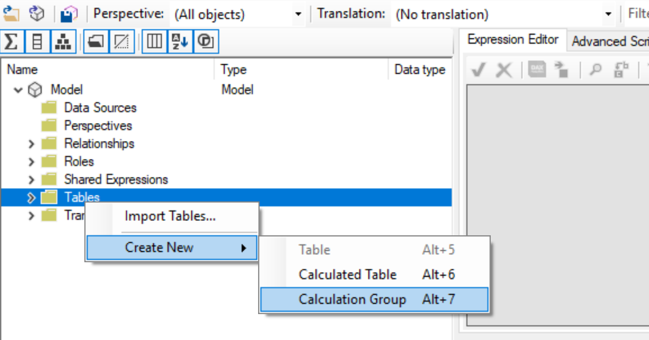
Calculation groups and many-to-many relationships are currently engine-only features. SSDT support will come before SQL Server 2019 general availability. In the meantime, you can use the fantastic open-source community tool Tabular Editor to author calculation groups. Alternatively, you can use SSAS programming and scripting interfaces such as TOM and TMSL.
Pace of delivery
We think you will agree the AS engine team has been on a tear lately. This is the same team that recently delivered, or is currently working on, the following breakthrough features for Power BI.
- Arguably the biggest scalability feature in the history of the AS engine: aggregations
- Policy-based incremental refresh
- Opening the XMLA endpoint to bring AS to Power BI
Calculation groups is yet another monumental feature delivered in a relatively short period of time. It demonstrates Microsoft’s continued commitment to enterprise BI customers.
Download Now
To try SQL Server 2019 CTP 2.3, find download instructions on the SQL Server 2019 web page. Enjoy!
0 Comments on "What’s new for SQL Server 2019 Analysis Services CTP 2.3"